"A picture is worth a thousand words" is an English idiom. It refers to the notion that a complex idea can be conveyed with just a single still image or that an image of a subject conveys its meaning or essence more effectively than a description does.
This idiom can also be applied to software programming. Indeed, you can easily understand a mini project by exploring its source code. However, a large project can quickly become complex and difficult to understand. In such cases, it’s better to visualize the source code using graphs and diagrams to make it easier for developers to understand.
Let’s explore some useful diagrams provided by CppDepend for understanding a codebase.
I - Treemap diagram
Treemapping is a method for displaying tree-structured data by using nested rectangles. The tree structure used in the CppDepend treemap is the usual code hierarchy:
- C/C++ projects contain namespaces,
- Namespaces contain types,
- Types contain methods and fields.
With a treemap, rectangles represent code elements. The level option determines the type of code element represented by each unit rectangle. The level option can take 5 values: project, namespace, type, method and field. The two screenshots below show the same code base represented with the type level on the left and the namespace level on the right.
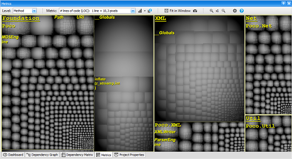
The Code Metric option of the treemap determines the size of rectangles. For example, if the level is set to type and the metric is set to number of lines of code, each unit rectangle represents a type, and the size of a unit rectangle is proportional to the number of lines of code of the corresponding type.
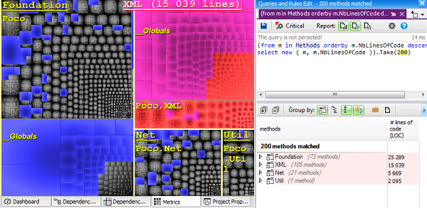
If a CQLinq query is currently being edited, the set of code elements matched by the query is shown on the treemap as a set of blue rectangles. In the screenshot below, a CQLinq query matches the 200 largest methods. Here the treemap level is method and the metric is number of lines of code. As expected, we can see that the blue rectangles represent the 200 largest unit rectangles of the treemap.
The screenshot below also shows that the currently selected code element (here the project XML) is shown as a red rectangle on the treemap.
Common Scenarios
By choosing an appropriate combination of metric and level values, the Metric View helps you see patterns that would be hard to spot in other ways. Too Big, Too Complex CppDepend provides many code metrics to spot overly large and overly complex code. Methods with too many parameters, variables, lines of code, or excessive cyclomatic complexity should be avoided. The same applies to types with too many lines of code.
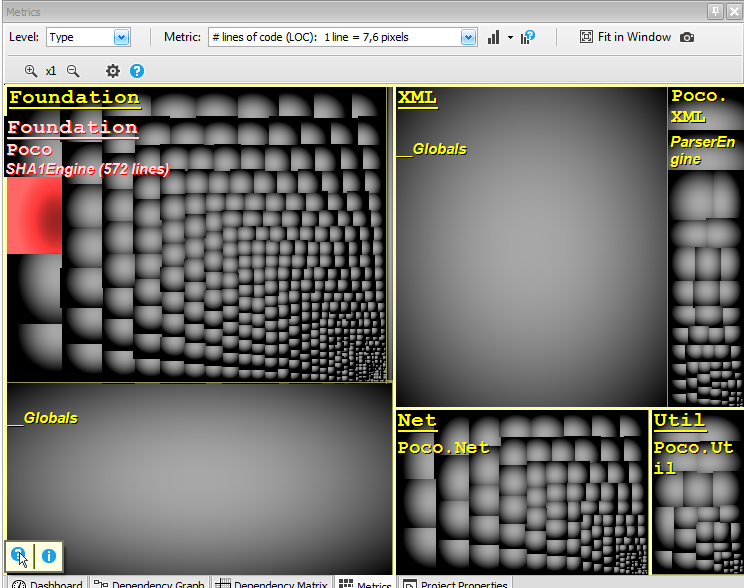
In the screenshot below, the treemap level is set to type and the metric is number of lines of code. Large rectangles represent the large types of the code base. Hovering over a rectangle shows the metric values for the type, here the type’s number of lines of code. Clearly, code treemapping not only helps spot overly large and overly complex code elements, but also helps compare their respective sizes and complexity.
Flaw Localization
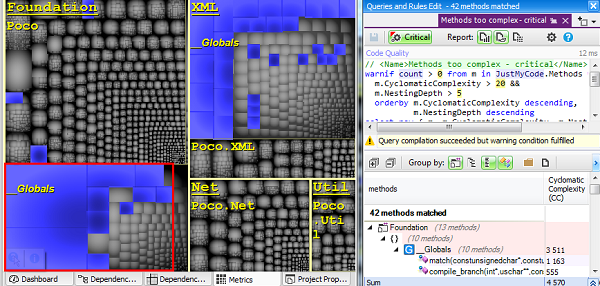
In the screenshot below, we use a CQLinq query to find methods with too many parameters and variables. Blue rectangles show the matched methods on the treemap. The interesting point here is that some matched methods seem to be grouped. Because the treemap is a hierarchical view, if a set of code elements is grouped, it means that the code elements belong to the same parent. And indeed, the 12 grouped methods here belong to the same type.
Identifying the parent types of these 12 methods would have been difficult without treemapping. Now the code quality reviewer can focus on this region, which seems to contain more flaws than other parts of the code base.
Top-Down Code Exploration
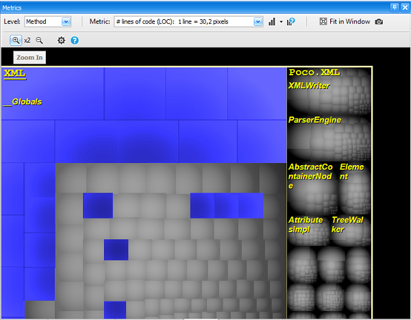
The CppDepend treemap metric view supports zoom-in and zoom-out. This makes it easy to zoom in on a particular project, namespace or class. This can be especially useful for exploring and comparing the volume of components in terms of lines of code.
By no means should productivity be measured in terms of lines of code. However, counting lines of code has proven to be a useful metric for accurately estimating software, given the context of an organization. The codebase features are organized into assemblies, namespaces, and types. With treemapping, these artifacts become rectangles that sit side by side. Rectangle areas, and hence feature weight, can be compared visually. Being able to periodically explore code size through treemapping is a unique way to build an accurate sense of feature weight and feature cost.
Try the experiment of visualizing a treemap of a code base you know well, and you’ll be surprised to discover unexpected feature sizes.
Code Structure Observations
Choosing to use the Metric View with a metric other than volume (lines of code, number of parameters for methods…) or complexity can reveal interesting observations.
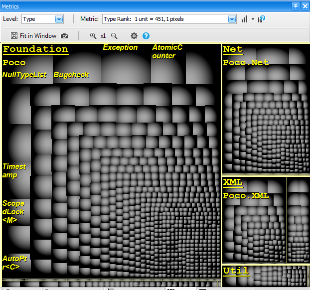
The ranking metric is a code metric that measures the popularity of a type or a method in a code base. Using treemapping with the ranking metric gives a clear view of where popular types are declared. This quickly reveals what is important in the codebase.
The screenshot below shows the types of the Microsoft DLR (Dynamic Language Runtime) code base treemapped with the ranking metric. The treemap indicates that CallSite and Expression are popular concepts of the DLR, and this is indeed the case.
The same kind of interesting Code Structure Observations can be made with code metrics such as Afferent/Efferent coupling or Level.
II - Dependency Graph
CppDepend offers a wide range of facilities to help users explore an existing code architecture using the dependency graph. Here are the most popular code exploration scenarios: Call Graph
CppDepend can generate any call graph you need using a two-step process.
- First: ask for the direct and indirect callers/callees of a type, a field, a method, a namespace or a project. The effect is that the following CQLinq query is generated to match all requested callers or callees.
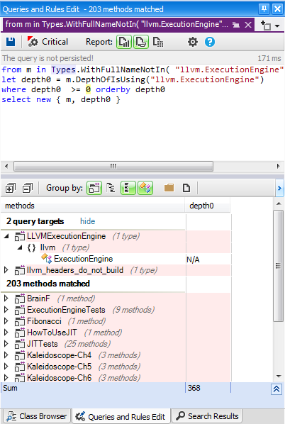
- Notice that, in the CQLinq query result, the metric DepthOfIsUsing/DepthOfIsUsedBy shows the depth of usage (1 means direct, 2 means using a direct user, etc.). The CQLinq query can easily be modified to only match indirect callers/callees with a certain condition on the depth of usage. Notice also that the requested callers/callees are not necessarily of the same kind as the code element concerned. For example, here we ask for methods that use a type directly or indirectly.
- Second: once the CQLinq query matches the set of callers/callees the user wants, the set of matched results can be exported to the dependency graph. This displays the desired call graph.
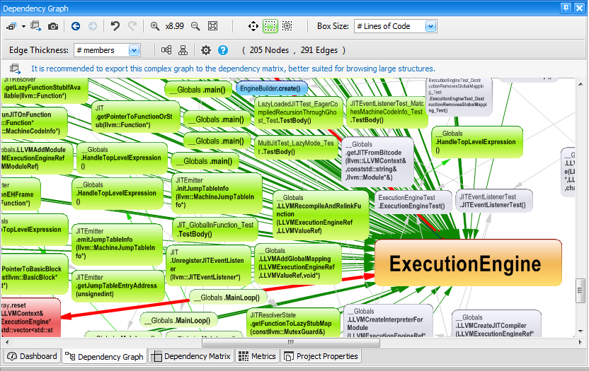
Class Inheritance Graph
To display a class inheritance graph, the same two-step procedure shown in the previous section (on generating a call graph) must be applied.
- First: generate a CQLinq query asking for the set of classes that inherit from a particular class (or that implement a particular interface). Here, the following CQLinq query is generated:
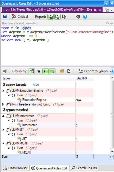
- Second: export the result of the CQLinq query to the dependency graph to show the desired inheritance graph.
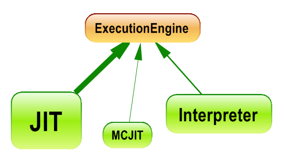
Coupling Graph
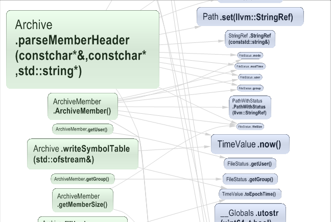
You might need to know exactly which code elements are involved in a particular dependency, especially when you need to anticipate the impact of a structural change. In the screenshot below, the CppDepend Info panel describes a coupling between 2 projects.
By pointing at a cell in the dependency matrix, it tells you that X types of a project A are using Y types of a project B. Notice that you can change the Weight on Cell option to # methods, # members or # namespaces if you need to measure coupling in terms of something other than types.
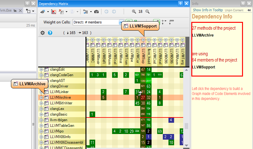
Simply left-clicking the matrix cell shows the coupling graph below.
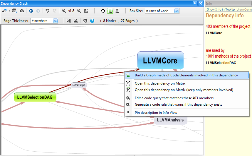
A coupling graph can also be generated from an edge in the dependency graph. Here, you can adjust the Edge Thickness option to something other than # type.
Path Graph
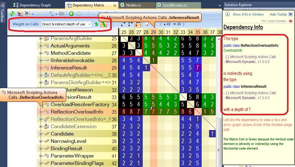
If you want to investigate a path or dependency cycle between two code elements, the first thing to do is to display the dependency matrix with the option Weight on Cells: Direct & indirect depth of use.
Blue and green matrix cells will represent paths, while black cells will represent dependency cycles. For example, here the Info panel tells us that there is a path of minimum length 7 between the 2 types involved.
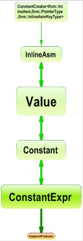
Simply left-clicking the cell shows the path graph below.
All Paths Graph
In certain situations, you’ll need to know about all paths from a code element A to a code element B. For example, here the Info panel tells us that there is a path of minimum length 2 between the 2 types involved.
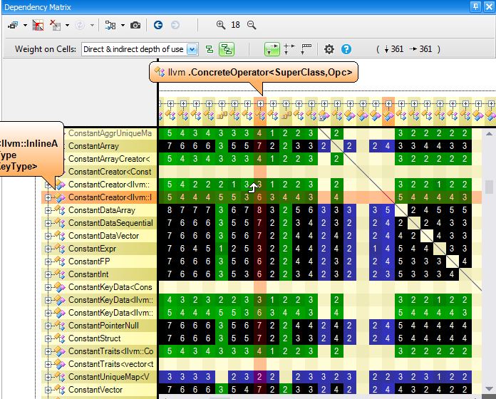
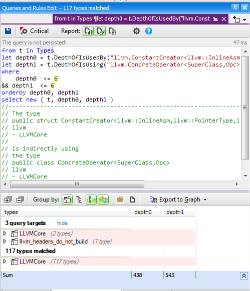
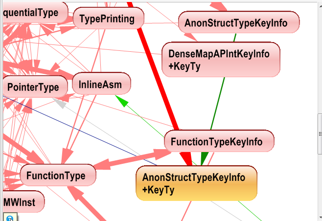
Finally, exporting the 12 types matched by the CQLinq query to the graph shows all paths from A to B.
Cycle Graph
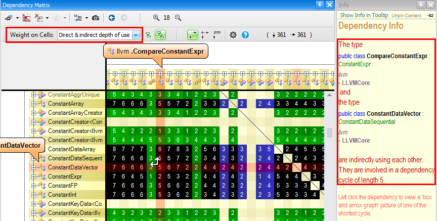
As we explained in the previous section, to deal with dependency cycle graphs, the first thing to do is to display the dependency matrix with the option Weight on Cells: Direct & indirect depth of use. Black cells then represent cycles.
For example, here the Info panel tells us that there is a dependency cycle of minimum length 5 between the 2 types involved.
Simply left-clicking the cell shows the cycle graph below.
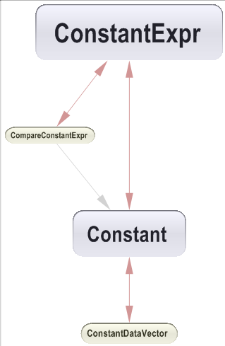
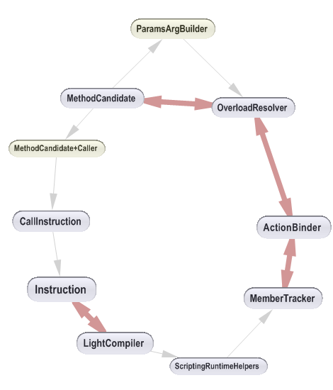
Note that obtaining a clean, “rounded” dependency cycle like the one shown above is the exception rather than the rule.
Often, exhibiting a cycle will result in a non-‘rounded’ graph like the one shown below. In this example, the minimum length of a cycle between the 2 types involved (in yellow) is 12. Count the number of edges crossed from one yellow type to the other, and you’ll get 12. You’ll see that some edges are counted more than once.
III - Dependency Structure Matrix
Large Graph visualized with Dependency Structure Matrix
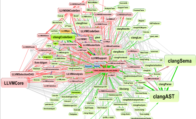
Here, we’d like to underline the fact that when the dependency graph becomes unreadable, it is worth switching to the dependency matrix. Both the dependency graph and the dependency matrix coexist because:
- The dependency graph is intuitive but becomes unreadable as soon as there are too many edges between nodes.
- The dependency matrix takes time to understand, but once mastered, you’ll see that the dependency matrix is much more efficient than the dependency graph for exploring an existing architecture. More information on dependency matrix readability can be found in Identify Code Structure Patterns at a Glance
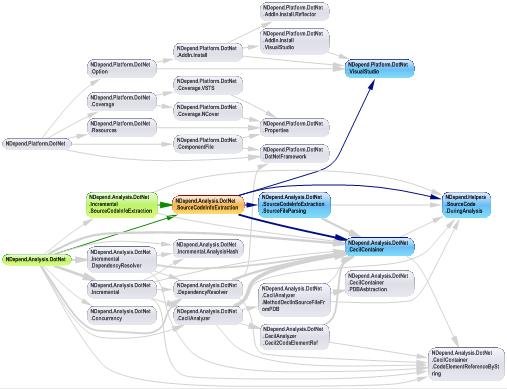
To illustrate the point, below are the same dependencies between 77 namespaces shown through a dependency graph and a dependency matrix.
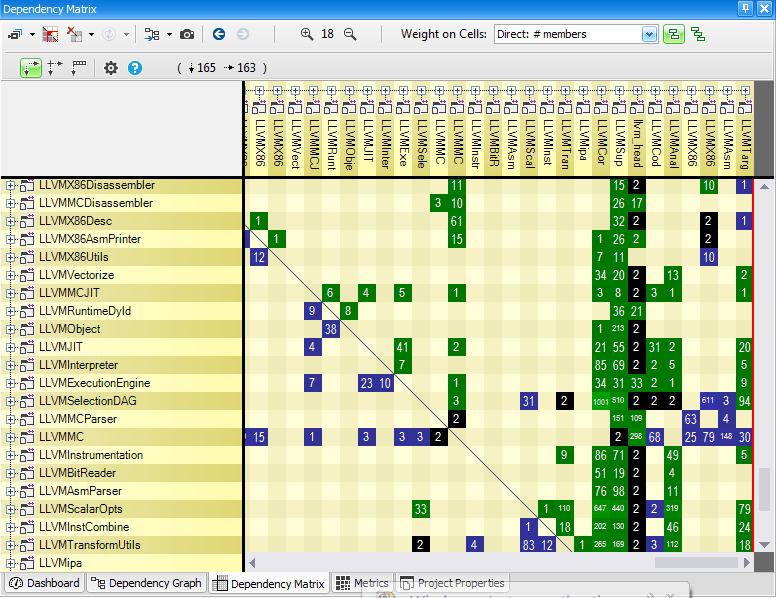
The DSM (Dependency Structure Matrix) is a compact way to represent and navigate across dependencies between components. For most engineers, talking about dependencies means talking about something that looks like this:
DSM is used to represent the same information as a graph.
- Matrix header elements represent graph boxes
- Matrix non-empty cells correspond to graph arrows.
As a consequence, in the snapshot below, the coupling from Net to Foundation is represented by a non-empty cell in the matrix and by an arrow in the graph.
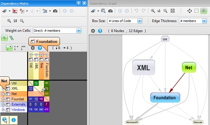
Why use two different ways — graph and DSM — to represent the same information? Because there is a trade-off:
- A graph is more intuitive but can become totally incomprehensible when the number of nodes and edges grows (a few dozen boxes can be enough to produce an overly complex graph)
- DSM is less intuitive but can be very efficient at representing large and complex graphs. We say that DSM scales better than graphs.
Once one has understood DSM principles, one typically prefers DSM over graphs to represent dependencies. This is mainly because DSM makes it possible to spot structural patterns at a glance. This is explained in the second half of this document.
CppDepend offers context-sensitive help to educate the user about what he sees on the DSM. CppDepend’s DSM relies on a simple 3-color scheme for DSM cells: blue, green and black. When hovering over a row or a column with the mouse, the context-sensitive help explains the meaning of this color scheme:
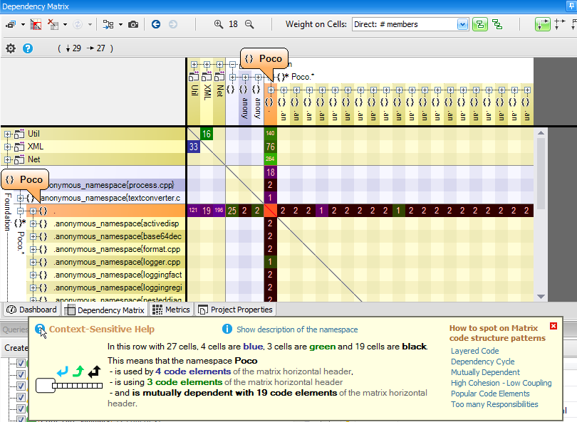
A non-empty DSM cell contains a number. This number represents the strength of the coupling represented by the cell. The coupling strength can be expressed in terms of the number of members/methods/fields/types or namespaces involved in the coupling, depending on the current value of the Weight on Cells option. In addition to the context-sensitive help, the DSM also offers an Info panel that explains the coupling with a plain-English description:
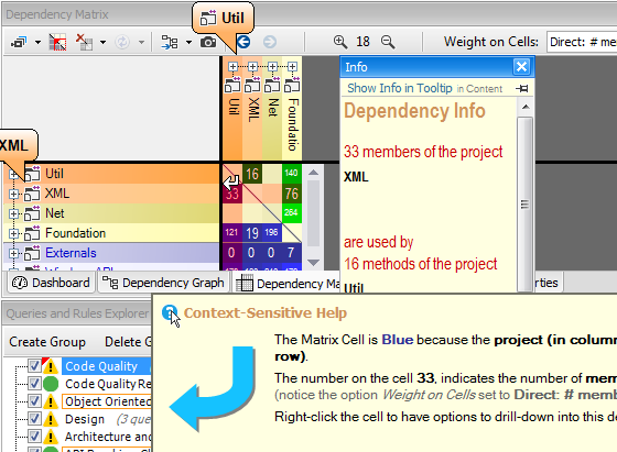
CppDepend's DSM comes with numerous options to try:
- It has numerous facilities for digging into dependency exploration (a parent column/row can be opened, cells can be expanded…)
- It can handle square symmetric DSMs and rectangular non-symmetric DSMs
- Horizontal and vertical headers can be bound together to always have a square symmetric matrix
- It comes with the Indirect usage option, where cells show direct and indirect usage
- The vertical header can contain tier code elements
- ...
It is recommended to try all these features yourself, by analyzing dependencies in your code base. Identify Code Structure Patterns on a Matrix
As explained in the introduction, DSM has the particularity of offering easy identification of popular code structure patterns. Let’s present the most common scenarios: Layered Code One pattern made obvious by a DSM is a layered structure (i.e. an acyclic structure). When the matrix is triangular, with all blue cells in the lower-left triangle and all green cells in the upper-right triangle, it shows that the structure is perfectly layered. In other words, the structure doesn’t contain any dependency cycle.
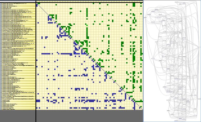
On the right part of the snapshot, the same layered structure is represented with a graph. All arrows have the same left-to-right direction. The problem with graphs is that the graph layout doesn’t scale. Here, we can barely see the big picture of the structure. If the number of boxes were multiplied by 2, the graph would be completely unreadable. On the other hand, the DSM representation wouldn’t be affected; we say that DSM scales better than graphs.
Side note: interestingly enough, most graph layout algorithms rely on the fact that a graph is acyclic. To compute the layout of a graph with cycles, these algorithms temporarily discard some dependencies to deal with a layered graph, and then append the discarded dependencies at the last step of the computation. Dependency Cycle If a structure contains a cycle, the cycle is displayed by a red square on the DSM. We can see that inside the red square, green and blue cells are mixed across the diagonal. There are also some black cells that represent mutual direct usage (i.e. A is using B and B is using A).
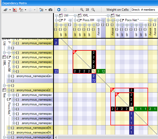
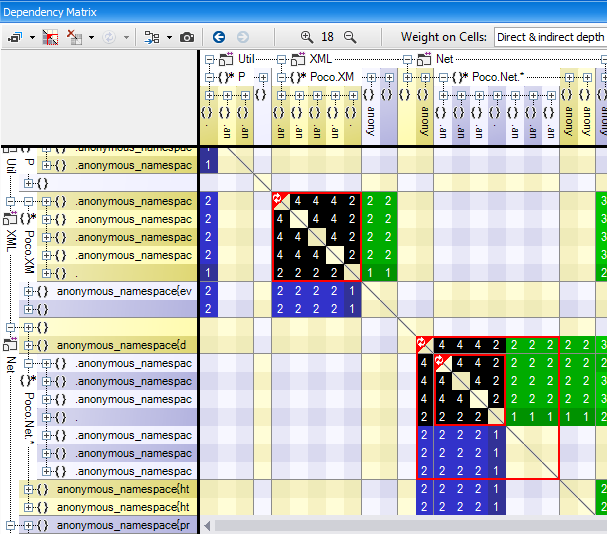
CppDepend’s DSM comes with the unique Indirect Dependency option. An indirect dependency between A and B means that A is using something, that is using something, that is using something … that is using B. Below, the same DSM with a cycle is shown in indirect mode. We can see that the red square is filled with only black cells. It simply means that for any elements A and B in the cycle, A and B are indirectly and mutually dependent.
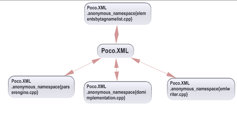
Here is the same structure represented with a graph. The red arrow shows that several elements are mutually dependent. But the graph is of no help in highlighting all the elements involved in the parent cycle.
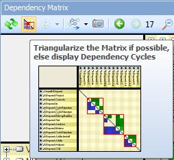
Notice that in CppDepend we provide a button to highlight cycles in the DSM (if any). If the structure is layered, this button triangularizes the matrix and keeps non-empty cells as close as possible to the diagonal.
High Cohesion – Low Coupling
The idea of high cohesion (within a component) / low coupling (between components) is popular nowadays. But if you cannot measure and visualize dependencies, it is hard to get a concrete evaluation of cohesion and coupling. DSM is good at showing high cohesion. In the DSM below, an obvious square aggregate around the diagonal is displayed. It means that the elements involved in the square have high cohesion: they are strongly dependent on each other. Moreover, we can see that they are layered since there is no cycle. They are certainly candidates to be grouped into a parent artifact (such as a namespace or an assembly).
On the other hand, the fact that most cells around the square are empty indicates low coupling between the elements of the square and other elements.
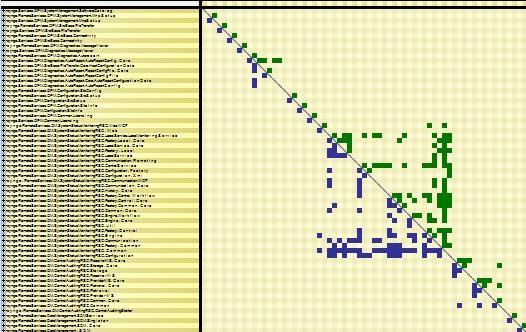
In the DSM below, we can see 2 components with high cohesion (upper and lower squares) and pretty low coupling between them.
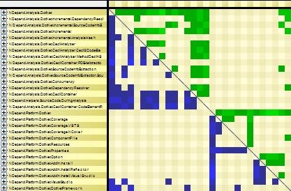
When refactoring, having such an indicator can be very useful to know whether there are opportunities to split coarse components into several more fine-grained components.
Too Many Responsibilities
The Single Responsibility Principle (SRP) is getting popular in the software architects community nowadays. The principle states that a class shouldn’t have more than one reason to change. Another way to interpret the SRP is that a class shouldn’t use too many different other types. If we extend the idea to other levels (assemblies, namespaces and methods), then certainly, if a code element uses dozens of different other code elements (at the same level), it has too many responsibilities. The term God class or God component is often used to describe such a piece of code.
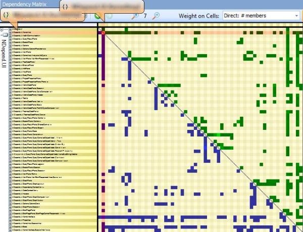
DSM can help pinpoint code elements with too many responsibilities. Such a code element is represented by columns with many blue cells and rows with many green cells. The DSM below exposes this phenomenon.
Popular Code Elements
A popular code element is used by many other code elements. Popular code elements are unavoidable (think of the String class for example), but a popular code element is not a flaw. It just means that in every code base there are some central concepts represented by popular classes
A popular code element is represented by columns with many green cells and by rows with many blue cells. The DSM below highlights a popular code element.
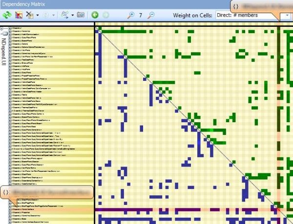
Something to notice is that when you keep your code structure perfectly layered, popular components are naturally kept at a low level. Indeed, a popular component cannot de facto use many things: because popular components are low-level, they cannot use something at a higher level. This would create a dependency from low-level to high-level, which would break the acyclic property of the structure.
Mutually Dependent
You can see the coupling between 2 components by right-clicking a non-empty cell and selecting the Open this dependency menu.
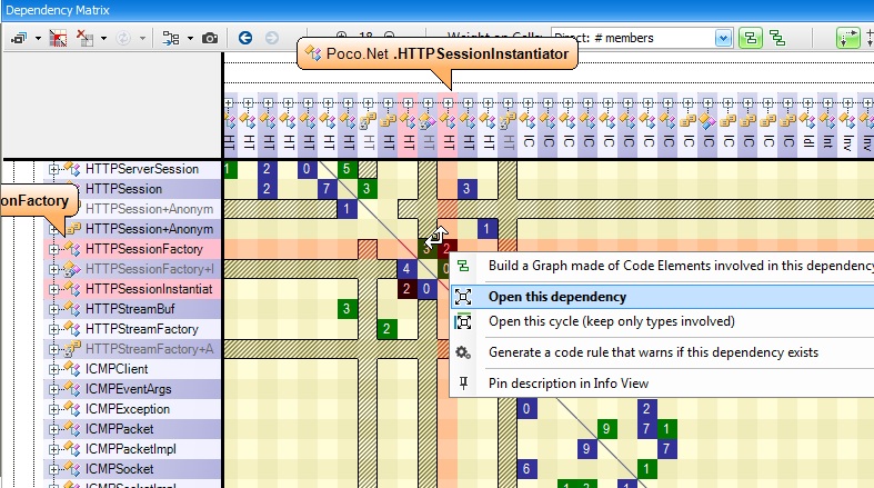
If the opened cell is black, as in the snapshot above (i.e. if A and B are mutually dependent), then the resulting rectangular matrix will contain both green and blue cells (and possibly black cells as well), as in the snapshot below.
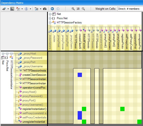
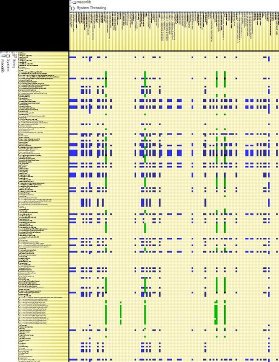
In this situation, you’ll often notice a deficit of green or blue cells (3 blue cells for 1 green cell here). This is because even if 2 code elements are mutually dependent, there is often a natural level order between them. For example, consider the System.Threading namespace and the System.String class. They are mutually dependent; they both rely on each other. But the matrix shows that Threading is much more dependent on String than the opposite (there are many more blue cells than green cells). This confirms the intuition that Threading is at a higher level than String.